Guest Post: An Explanation of Yahoo’s Standard Deviation Stat Filter

By Johnny Guestpost

A few years ago, Yahoo introduced a new option for filtering its player list in fantasy hockey: standard deviation or “std dev”.  This may have gone under the radar for a lot of people but it can actually be a very useful tool, especially in stat-category leagues, if you know how to use it. 

Let’s say you’re going through the available player list on Yahoo, perhaps looking for a player to replace a player on IR or IR+.  You’re no stranger to the process – maybe you’re a perennial Kris Letang owner, or maybe there were years past where you were convinced this was Rick DiPietro’s year.  You know to check out the average stats in addition to the total stats to find players who are scoring at a good clip, but aren’t highly ranked overall because an injury or a slow schedule has resulted in fewer games played.  You’ll check out the Last 30/14/7 Days lists to see who’s been hot.  You might even check the Opponents list, because your IR player will be coming back soon and you’d like someone short-term, who’s going to be playing the most games before your IR player returns.

But now, Yahoo also has the std dev option.  Yahoo introduced this feature fairly quietly, with a less than fulsome explanation:

 

So what is this new way to look at player stats?  In the most basic terms, the standard deviation is the distance from the average value for that category, taking into account how spread apart the values in that category are.  The first basic principle is that players who score greater than the average in any given category will have a positive std dev value for that category, while players that score less than the average in a category will have a negative std dev value for that category.  It’s useful to think of a curve here.

The x-axis (horizontal) is the number of goals scored.  The y-axis (vertical) is the number of players that have scored that many goals.  The average is somewhere in the middle of the curve, such that players that fall to the right will have positive std dev values, and players that fall to the left will have negative  values.   So far, pretty simple right? (i.e. positive number = good; negative number = bad).

But, how steep or shallow the curve is will affect how large the std dev values are.  Exactly how positive or how negative the std dev value will be depends on the rest of the player population’s scoring in the category.

Say a player has 25 goals.  In the above graph, where most have between 0 and 8 goals, our 25-goal scorer would have an std dev value of slightly higher than 2 (far ahead of the pack). But let’s look at another example, where the goal scoring is a bit more spread out (as you can see on the horizontal axis), and the number of players scoring nothing is reduced (as you can see on the vertical axis):

 

 In this case, “most” players are scoring between 0 and 12 goals, and so our 25 goal scorer’s std dev value is still positive, but is a bit lower, at just over 1 (because the range of values that most players are scoring is wider, and thus our scorer isn’t doing as well as compared to this group).

To dispel a common myth, the std dev value is not based merely on how many other players a given player beats.  It’s not based simply on percentile, where a player is given a higher value because they are better than 99% or 99.5% of the other players (indeed, in our above example, our 35-goal scorer could be the league leader at the time, thus being ahead of everyone, but has a lower std dev value when the scoring values for the players beneath him are more spread out).  This confusion arises because percentile can often be calculated from standard deviation under certain circumstances, so many believe they go hand-in-hand.  This is not always the case.

To illustrate, let’s look at 2014-2015’s top five goal scorers, and their corresponding std dev values.

Total Goals:

Std Dev Values:

If these values were based solely on the number of players a particular player beats, then we would see a predictable jump in std dev value from player to player independent of anything else (since as we go up the list, each player is ahead of one additional player in goals rank).  Instead, we see jumps that follow goals.  Tavares to Nash is a large 0.5 jump (a large four goal difference), followed by a modest 0.12 from Nash to Stamkos (a modest one goal difference), followed by a tremendous 1.21 jump from Stamkos to Ovechkin (a tremendous ten goal difference).

This is one reason that std dev value is useful; if it were based merely on rank, Ovechkin would have the same listed value in the top spot whether he had 53 goals or 530 goals.  Obviously, a player with more goals is going to be more valuable regardless of rank, so we want that taken into account.  Std dev value accounts for how well a player does in addition to how much better that player has done as compared to the herd.

You might be thinking, “Hey, I know another stat that gets higher as a player scores more goals:  The goals category.”  You’d be right, too.  There isn’t much new information to be gleaned from this one category.  Then what is the point of these numbers, and why are they more useful than just plain stats?

The key is the difference we saw when we looked at the different std dev values for the steep and shallow goal scoring bell curves above.  When we’re looking just at goals, for example, the curve is either going to be steep or shallow, based on what goal scoring is like at the time.  But in fantasy hockey, we want to look at goals and assists and shots and many other categories and figure out which players are better than others over all of the categories as a whole.  Each of these categories is going to have its own curve and to compare the different stats, we need to take into account the curve for each stat.

At its heart, a standard deviation is a measure of variance (how spread out the values are), but why it’s useful to us is because it’s a standard.  The length of a road (like the fantasy value of a hockey player) can be measured in a number of ways, like miles (goals) or kilometers (assists).  Driving down a road, you’d pass kilometer markers much more frequently than you would if they were mile markers (just like in hockey you will see many more assists awarded than goals).  Miles and kilometers are easy to just convert to each other because the length of a mile and kilometer don’t change.  But the average amount of goals and assists being scored each hockey season does fluctuate (and players are accumulating values in both categories – as if you were driving down a road that kept switching between mile markers and kilometer markers).  When you want to compare or add one stat to another, we need to have a standard unit takes into account the variance of each category.   Using standard deviation, we can compare how well a player did in each category against such a standard unit.  We can look at a player’s std dev value for goals and recognize that it has the same meaning as the std dev value in assists or shots on goal, because it takes into account the variance within those individual stats (i.e. std dev has the same meaning despite the fact that curves/distributions for each stat are different).

This is very important in a stat-categories league, where each scoring category has the same meaning: 1 win.  A win in goals is worth the same as a win in assists and worth the same as a win in shots on goal.  Therefore, a player who can single-handedly win the goals category is going to be worth as much as one who can single-handedly win the assists category.  By looking at only at the raw stats, we can’t clearly see what’s worth more: scoring 30 goals or having a 50 assists.  It’s an apples to oranges comparison.  A 4.3 std dev value in goals vs. a 5.4 std dev value in assists is closer to an apples to apples comparison.  It tells us that the second player is much better at scoring assists than the first player is at scoring goals.  Once we have each category expressed in the standard, we can add them and determine who’s contributing the most value from their roster slot.  Is a 20 goal, 40 assist player contributing more than a 25 goal, 35 assist player?

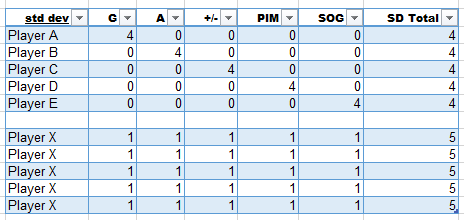
Here’s an example pulling numbers from the real world to illustrate that this can work using five scoring categories, G/A/plus-minus/PIM/SOG.  Let’s take 5 players (call them Player A through E) who excel in only one category, and we’ll give them an std dev value of 4 in that category.  They are perfectly average in every other category, earning them a zero std dev value in those.  Each player therefore has a total std dev value of 4 across all categories.  We’ll compare them to a team comprised of five copies of Player X, who is one standard deviation better than average (std dev value of 1) in every category.  This player therefore has a total std dev value of 5 across all categories.  The table below shows what the data would look like if you pulled up their std dev value from Yahoo.

Next, we can take real-world values from 2014-2015 (rounded a bit) to see what these std dev values correspond to, as shown in the following table.

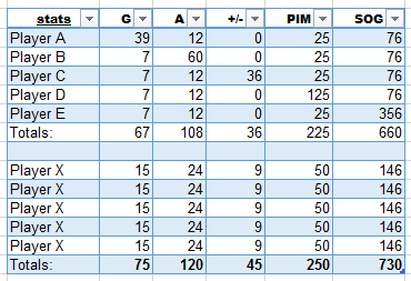
For example, four standard deviations from the mean in goals corresponded to 39 goals that year.  One standard deviation away would be 15, and average would be 7.  Therefore, in the goals column, the mean (std dev 0) is worth 7 goals.  The standard deviation in goals that year was 8, meaning that every 1 std dev point translates into 8 additional goals.  In assists, the mean is 12.  The standard deviation for assists that year was also 12, so for every std dev point, the player got 12 additional assists.  In this case, every 8 goals a player scored was worth as much as every 12 assists they scored.  Each category is normalized.  When we compare the totals for each team as if they were matched, Team X (the players that contributed better than average in every category) swept Team ABCDE (the one-category specialists).  Why? Because in each category the total std dev values (5) were greater than for Team ABCDE (4).   Would it be in Team ABCDE’s interest to trade (or add/drop) one of its players for a Player X?  Certainly.   If they did, they’d catch up to tie Team X in 4 of the categories (while continuing to lose the category of the specialist they dropped).   Decisions in fantasy hockey aren’t always this clear-cut, but this example illustrates how std dev values can help us figure out whether players are more useful to a fantasy team than others by adding their total std dev values.

Let’s look at some of the top players in std dev value in a sample league last year to talk about the cons of using standard deviation as Yahoo presents it:

First thing you notice is goal scorers dominate the list.  That makes sense for this league; goal scorers will usually have plenty of SOG behind them, and by sheer probability will have more GWG.  Another thing you might notice is most have a high SHP rating, resulting from scoring 5 SHP each on the season.  This can be a pro or a con when you’re doing research.  Due to the rare nature of SHP, a single SHP can win you the category for the week.  Therefore, a player that can single-handedly win a category deserves a higher ranking…if you’re judging past performance.

As personal opinion, past SHP scoring alone isn’t indicative of future scoring, and the future is the whole reason we as fantasy owners look to player stats.  At the very least, it shows that this player plays on the penalty kill.  It won’t tell you whether that player scored shorthanded because it was an end of game, open-net lay-up or because they are regularly intercepting high slot passes and getting frequent shorthanded breakaways.

If we’re looking to judge players for the future, a lopsided stat like SHP might be artificially inflating their rank.  A possible simple fix is to simply subtract that value from the total, thereby ignoring it.   Or, if you find you can’t predict it at all, go for the nuclear option and petition your commissioner to rework their chosen categories).

The next thing you might notice are the positions of the players – all happen to be wingers.  Centers do populate the ranks a decent amount past the list above, but defensemen don’t show up until rank 24, with a tight group of about five defenseman grouped together.  The following list is filtered for only defensemen.

Much lower numbers than our top five wingers.  The std dev rating gives zero consideration to positional scarcity.  That still falls on you, the fantasy manager, but std dev makes it a little easier for you.

The last consideration is games played.  You’ll see GP* with the asterisk above, meaning it’s not a fantasy scoring category and not included in the std dev value.  Yahoo’s std dev is calculated based on raw totals for the season.  Byfuglien and Letang have significantly fewer games played, with 69 each.  If they played for a full season and scored at the same pace, they would top the list easily.  Unfortunately it’s not as simple to extrapolate standard deviation values without extrapolating each underlying category stat, but in tight groups like the list above you can kind of sense where there are undervalued players.

In conclusion, std dev is not a one-stop shop for evaluating possible roster moves.  It has its drawbacks, and it is important to keep in mind what it is telling you when you’re using it.  But, so long as you have that understanding, it is a nice thing to have in your fantasy toolbox.